Show Chart For Selected Row via Hyperlink Excel VBA Macro

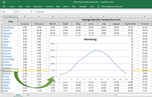
In this post we learn how to add a chart to show the data in the selected row using Excel VBA macros. We add a hyperlink to each row first, which triggers the procedure to show the chart. Thus, the macro consists of two procedures, one to add the hyperlinks, and another to add a chart every time a hyperlink is clicked. Additionally, the macro requires two event procedures to allow following the hyperlink, and to remove the chart when any other cell is selected. That makes the chart show up for each selected row each time.

Macro code:

 

  Sub AddHyperlinks()

      Dim r As Integer, lr As Integer

 

      lr = ActiveSheet.Cells(Rows.Count, "A").End(xlUp).Row

 

      For r = 3 To lr

          ActiveSheet.Hyperlinks.Add Anchor:=Range("A" & r), Address:="", _

          SubAddress:="Sheet1!A" & r

      Next r

  End Sub

 

  Sub ShowChart()

      Dim r As Integer, chartobj As ChartObject

 

      r = ActiveCell.Row

 

      Set chartobj = ActiveSheet.ChartObjects.Add(250, 100, 450, 250)

 

      With chartobj.Chart

          .ChartType = xlLine

          .SetSourceData Source:=ActiveSheet.Range("B" & r & ":M" & r)

          .HasTitle = True

          .ChartTitle.Text = ActiveCell.Value

          .HasLegend = False

      End With

  End Sub

 

 

In module Sheet1:

 

  Private Sub Worksheet_SelectionChange(ByVal Target As Range)

      If ActiveSheet.ChartObjects.Count > 0 Then

          ActiveSheet.ChartObjects.Delete

      End If

  End Sub

 

  Private Sub Worksheet_FollowHyperlink(ByVal Target As Hyperlink)

       ShowChart

   End Sub

 

 

Macro explained:

The first procedure (AddHyperlinks) adds hyperlinks to all cells in column A. That’s where we have the name of the city in the example above. Here’s what we do in AddHyperlinks:

• We declare two integers to store each row number (r) and number of the last row with content (lr). We get the last row with content with the End and Row properties for cells in column A.
• Then we loop through the column and add a hyperlink to each cell. The Anchor of the hyperlink is the cell itself (the location where the hyperlink is added). The Address is not necessary for a location inside the document (or Excel file in this case). The Subaddress is set the cell itself (so it is the same as the anchor), and requires a worksheet reference (not an object reference). Thus, following the hyperlink selects the cell which hyperlink was clicked.

The second procedure (ShowChart) adds the chart upon clicking the hyperlink. But that requires an event procedure to handle the trigger (see later). Here’s what we do in ShowChart:

• We declare the row number variable again (r) and a ChartObject object variable (chartobj) to add and assign to the embedded chart in the active worksheet. As explained earlier, the hyperlink selects the row. Then, we can get the row number (r), with ActiveCell.Row.
• We add and set an embedded chart to the variable chartobj. The position of the chart is 250 points and 100 points from the left and top edges of the worksheet respectively, and it is 450 points wide and 250 high. This can be changed to whatever fits your screen or in some other position and with other dimensions altogether.
• Then we specify the chart type as a line chart, displaying the data in columns B to M for the selected row. We set the title to the value in the selected hyperlink cell (name of the city), and hide the legend. Other formatting can also be applied this way as needed.

Finally, we need to add two event procedures to the module Sheet1. The first event procedure is triggered when the selected cell or range changes, and it deletes the chart embedded in the worksheet (if any). The second event procedure calls the ShowChart procedure when a hyperlink is clicked.

 

This is how we show a chart for the selected row in Excel using VBA macros.

Other examples:

• How to Sort and Merge Groups In Table with Excel VBA macros
  
• How to Add Buttons To Delete Rows with Excel VBA macros
  
• How to Compare Two Workbooks with Excel VBA macros